Hierarchically Combined Queueing Petri Nets

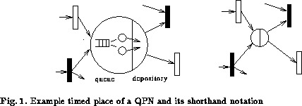
In the original QPN formalism [2] the timing aspects of a coloured GSPN [13] are extended by the option of integrating queues into places (see Fig. 1). Such a timed place consists of a queue and a depository for served tokens. Tokens being added to a timed place, after a transition firing, are inserted into the queue according to the queue's scheduling strategy. Each colour of tokens has an associated individual service time distribution of Coxian type. After service the corresponding token moves to a depository, where it is available to the place's output transitions. Tokens in a queue are not available for firing.

Every QPN can be analysed with respect to qualitative and quantitative aspects. The qualitative analysis of a QPN is completely based on the QPN's underlying coloured Petri net, where all timing aspects are neglected. The basis for a quantitative analysis of a QPN is its corresponding Markov chain. Every QPN describes a stochastic process. A state of this process is determined by the cartesian product of the state descriptors of all timed places and the number of coloured tokens within ordinary places. The initial marking of the QPN defines the initial state of its stochastic process under the assumption that initially all tokens contained in timed places are situated on the corresponding depository. The state space is partitioned into two types of states similar to GSPNs [1]: vanishing and tangible. A quantitative analysis can be performed with conventional techniques [2]. The complexity of a quantitative analysis is significantly reduced if the QPN has a hierarchical structure.

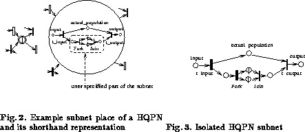
Hierarchically combined Queueing Petri nets (HQPNs) are obtained by a natural generalisation of the original QPN formalism. In HQPNs a timed place may contain a whole HQPN subnet instead of a single queue (cf. Fig. 2). Such a place is called a subnet place. A HQPN subnet might be a QPN subnet or again a HQPN comprising additional subnet places.

The HQPN subnet of a subnet place has a dedicated input and output place, which are ordinary places of a coloured Petri net. Tokens being inserted into a subnet place after a transition firing are actually added to the input place of the corresponding HQPN subnet. The semantics of the output place of a subnet place is similar to the semantics of the depository of a timed place: Tokens contained in the output place are available for the output transitions of the subnet place; tokens contained in all other places of the HQPN subnet are not available for the output transitions of the subnet place. The HQPN subnets we consider in this context have to observe the conditions given in the description of the hierarchical analysis approach. HQPNs can be analysed as flat models with respect to qualitative and quantitative aspects employing well-known algorithms of Petri net and Markov theory. In the sequel we concentrate on the new approach for quantitative analysis.

Integration of subnet places into the original QPN formalism leads to a hierarchical structure of a QPN model. Such a hierarchical structure can surely contain more than just two levels but for simplicity of notation we restrict ourselves in the following to a two-level hierarchy. Let high-level QPN (HLQPN) denote the upper level of a HQPN. The HQPN subnets of the subnet places in the HLQPN are denoted by low-level QPNs (LLQPNs).

The quantitative analysis employing this hierarchical structure, called structured analysis, comprises the following steps:

1. Generation of the HLQPN state space and transition matrix.
All subnet places of the HLQPN are replaced by the subnet's dedicated input and output places. Each input and corresponding output place is connected via a timed transition, which behaves like the output transition of the LLQPN and has a nonzero transition rate. We will call such a timed transition virtual since the firing rate might be chosen arbitrarily. The initial marking of the HLQPN is given by the initial marking specified on that level. The specification of the HLQPN is independent of the internals of the LLQPNs apart from their output transitions, which determine the input/output behaviour of the LLQPNs. Provided the HLQPN includes no timeless traps, which can be checked on the net level [2], we can determine its state space and transition matrix containing only tangible states. LLQPN specifications have to observe the restrictions given below.

2. Generation of the LLQPNs' state spaces and transition matrices.
For a structured analysis, the subnet integrated into a subnet place is restricted to HQPN subnets satisfying the following restrictions [7]:

1. The set of token colours are identical for the input and the output place. Arcs are not allowed which connect the dedicated output place with a transition of the subnet.
2. The macro state descriptor of the LLQPN, as needed for step 1, is given by a fixed set of places. In the current version of the QPN-Tool this set is determined by the places input and actual_population. Transition t_input is defined to behave like an identity function, so that transition t_output describes the behaviour of the HQPN subnet as seen in the HLQPN.
3. The subnet is structurally bounded, i.e. for any number of tokens entering the subnet, the number of all tokens in the subnet is always bounded above by some value . The modeller can check this restriction employing a local qualitative analysis of the isolated subnet (cf. Sec. 3), e.g. calculating a cover of positive P-invariants.
4. According to our assumptions about the influence of the HLQPN on the behaviour of a subnet we restrict this behaviour at the LLQPN level to a kind of single step behaviour: If a token enters the subnet (being fired onto the input place), no token can be fired onto the output place at the same (!) point of time.

Given these restrictions the state space and transition matrix for each LLQPN are generated in isolation (see Fig. 3). The behaviour of a LLQPN's environment is completely specified by the state transitions of the HLQPN determined in step 1.

In the quantitative analysis timed places can be viewed as special cases of subnet places where the queue forms the HQPN subnet and the output place is given by the depository of the timed place. A timed place trivially satisfies the above given restrictions. It can consequently be handled as a subnet place where the queue and the corresponding depository are considered as a LLQPN.