![]()
The following example demonstrates the advantages of the structured analysis of HQPNs compared to conventional techniques.
The HLQPN of our example system is shown in
Fig. 6:  workstations Proc_1,
  ,
Proc_5 with a local disk each, and a special diskless workstation
Manager with two processors and a joint processor sharing
scheduling strategy. All workstations are connected via a
bidirectional bus which has to be used exclusively.
,
Proc_5 with a local disk each, and a special diskless workstation
Manager with two processors and a joint processor sharing
scheduling strategy. All workstations are connected via a
bidirectional bus which has to be used exclusively.
The workstations Proc_1, , Proc_5 are identically
specified by the subnet given in Fig. 7: A
customer/token entering the subnet is forked into several jobs which
are processed at the CPU. Several disk accesses might be necessary
before a job completes its service at that workstation. A served
job is modelled by a token of appropriate colour on the place Done. If all corresponding jobs have completed their service, they
join again by firing transition t_output and the resulting
customer/token may leave the subnet.
The system is used for an iteration problem, each workstation calculates a specific part of the iteration vector. This part is transmitted to the Manager via the Bus. When the Manager has received all parts of the new iteration vector, it updates its local copy and distributes the updated vector to all workstations via broadcasting. We assume that calculation of the fixed point takes a huge number of iterations and therefore only consider the iteration process, neglecting all convergence issues in our model.
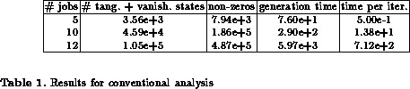
The model is analysed for an increasing number of jobs running on the workstations. All experiments were performed on a workstation with 16MB main memory and 48MB virtual memory, time is measured in seconds as real time which is a more appropriate measure than CPU time. Table 1 and 2 summarise the results for some configurations. We assume that all workstations are identical, thus in the structured analysis approach we need to generate only matrices for workstations with different populations. It can be seen that the size of the state space grows rapidly with an increasing number of jobs in the system. The first column contains the total number of jobs, the second column in table 1 and 2 the number of tangible + vanishing states and the number of tangible states, respectively. The number of tangible states is identical for the conventional and structured approaches, however, in the structured approach vanishing states are eliminated locally, such that only the tangible part of the complete state space is generated. The number of tangible states equals the state space size of the Markov chain. For the conventional approach first all states, tangible and vanishing, have to be generated, subsequently the vanishing states are eliminated. For a structured analysis only HLQPN and LLQPN state spaces have to be generated and vanishing states can be eliminated locally. The largest state space which has to be handled for a structured analysis is the HLQPN state space consisting of 272 tangible and 682 vanishing states. The LLQPN state spaces are all smaller for the above parameters. The time needed to compute the state space and to eliminate vanishing markings is given in column four. Apart from the smallest configuration with only 5 jobs, the structured approach is much faster, in spite of the strictly sequential implementation of the structured state space generation, which means that the generation process is started several times which increases the effort for smaller state spaces. The generation time for the structured approach is nearly independent of the state space size, whereas the generation time for the conventional approach depends heavily on the number of states to be generated and the number of vanishing states to be eliminated.
![]()
![]()
![]()
![]()
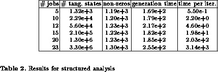
Column three contains the number of non-zero elements which have to be stored to represent the generator matrix. For the structured approach the number of elements is nearly invariant for an increasing number of jobs. On a first glance at table 2 it might be surprising that we need more elements for 12 than for 15 jobs; however, this is caused by the different workstation populations for 12 jobs which requires the storage of two sets of matrices, one for workstations with 2 running jobs, and one for workstations with 3 running jobs. For 15 jobs all workstations receive 3 jobs. The storage of iteration and solution vectors is the limiting factor of structured analysis. The conventional approach requires a huge number of elements to be stored, although the generator matrix is sparse and we use, of course, a sparse storage scheme. The storage of the generator matrix becomes the limiting factor of the conventional approach. We were able to handle up to 12 jobs with the conventional approach, which equals a model with slightly more than 100,000 states; for larger populations the elimination of vanishing markings exhausts available memory. The structured approach allows to handle models with up to 23 jobs and more than three millions tangible states and additional vanishing states which are never generated in the complete state space. Of course, the solution of such a model is time consuming, if vectors do not fit into main memory.
The time needed for one iteration of the vector with the iteration
matrix is given in column five for the
conventional and structured approach, respectively. It is obvious that
the structured approach takes a similar time for small state spaces
and is much faster for larger models. The latter is caused by the
extremely time consuming paging operations needed for the conventional method
whenever the
generator matrix does not fit into primary memory.
The time required for
a complete solution depends on the transition rates, the solution
technique, the initial vector and the required accuracy. However,
starting from an initial vector obtained by the approximation method as
described above, the model can be analysed for a rather wide variety
of parameters with between 40 and 300 iteration steps to yield an
estimated accuracy of  for the solution vector. Thus it is
possible to solve all models on a standard workstation, although the
analysis of the largest configuration would take quite long. Using
slightly more powerful machines would reduce the solution time to one
night.
for the solution vector. Thus it is
possible to solve all models on a standard workstation, although the
analysis of the largest configuration would take quite long. Using
slightly more powerful machines would reduce the solution time to one
night.
It should be noticed that the above model can be analysed more efficiently by exploiting symmetries in the model specification to generate first an exactly reduced Markov chain, which is afterwards solved using the structured approach. Examples for the reduction of a similar model are given in [3], the technique extends results on Stochastic Well-Formed Nets [10] and is described in [8]. Symmetry exploitation is currently not available in QPN-Tool, work towards an implementation is underway.